
A practical breakdown of the 10 AI search algorithms that appear most often in CS exams, coding interviews, and real production systems, with complexity data and study order.
Top 10 AI Search Algorithms Every CS Student Should Know
Search is the oldest and most reusable idea in artificial intelligence. Before neural networks, before transformers, before anything called a model, AI was defined as the systematic exploration of a space of possibilities. That definition still holds. A route planner, a chess engine, a Sudoku solver, a compiler register allocator, and an LLM decoding tokens with beam search are all doing the same thing: expanding candidate states, scoring them, and deciding which one to expand next.
This matters for a very practical reason. Most CS students learn search algorithms as isolated exam questions, memorize the pseudocode two days before the paper, and forget the tradeoffs. Then an interviewer asks why A star beats Dijkstra on a game map, and the answer does not come. The fix is understanding four properties for every algorithm: completeness, optimality, time complexity, and space complexity. Once you can recite those four for each algorithm below, you actually know search.
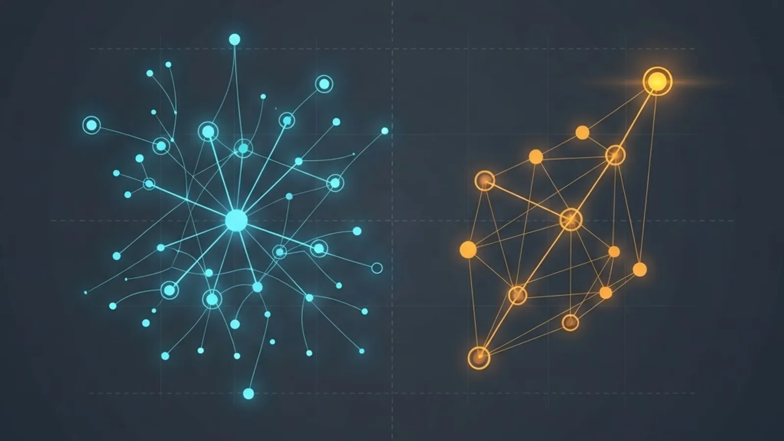
Quick Answer: Every CS student should know BFS, DFS, Depth-Limited Search, Iterative Deepening, Uniform Cost Search, Greedy Best-First, A star, Bidirectional Search, Minimax with Alpha-Beta Pruning, and Hill Climbing. These ten cover uninformed, informed, adversarial, and local search, and together they underpin pathfinding, planning, and game AI.
Key Terms Defined Before You Start
Get these five definitions right and every algorithm below becomes easier to reason about.
- State space: the set of all configurations reachable from the start state. A 3x3 sliding tile puzzle has 181,440 solvable states. The 4x4 version has roughly 10 trillion.
- Branching factor (b): the average number of successors per node. Chess averages about 35. Go averages about 250.
- Completeness: the algorithm is guaranteed to find a solution if one exists.
- Optimality: the algorithm is guaranteed to find the lowest-cost solution, not just any solution.
- Admissible heuristic: a heuristic h(n) that never overestimates the true remaining cost. Admissibility is the exact condition that makes A star optimal.
1. Breadth-First Search (BFS)
BFS expands all nodes at depth d before touching depth d+1, using a FIFO queue. It is complete, and it is optimal when every edge has identical cost, because the first time it reaches the goal it has done so in the fewest possible moves.
The catch is memory. Time and space are both O(b^d). With a branching factor of 10 and a depth of 12, that is roughly a trillion nodes in the frontier. This is why BFS is excellent for shortest-hop problems like social graph degrees of separation or word ladders, and useless for deep search trees.

Use it when: edges are unweighted and the solution is shallow.
2. Depth-First Search (DFS)
DFS follows one branch to its end before backtracking, using a LIFO stack or recursion. Its defining advantage is space: O(bm) where m is maximum depth, which is linear rather than exponential. That single property is why DFS powers topological sorting, cycle detection, strongly connected components, and constraint backtracking.
Its weakness is equally sharp. DFS is neither complete nor optimal on infinite or cyclic graphs, because it can descend an infinite branch forever. Always add a visited set on graphs.
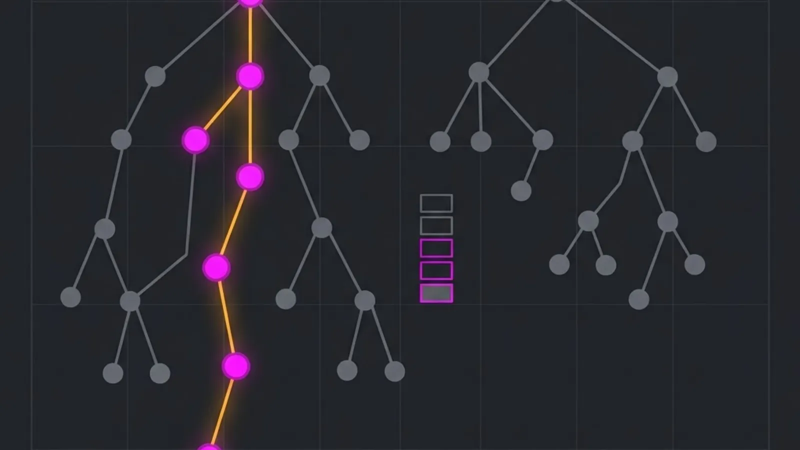
Use it when: memory is tight, solutions are deep, or you need structural graph properties.
3. Depth-Limited Search (DLS)
DLS is DFS with a hard cutoff at depth L. It fixes the infinite-branch problem and keeps DFS memory behavior. The tradeoff is that it becomes incomplete in a new way: if the shallowest solution sits below L, DLS reports failure even though a solution exists.
DLS is rarely the final answer. Its real value is as the building block for the next algorithm, and as the mechanism behind fixed-depth game engines that must return a move inside a time budget.
4. Iterative Deepening Depth-First Search (IDDFS)
IDDFS runs DLS with L = 0, 1, 2, 3 and upward until a solution appears. It sounds wasteful and it is the opposite. Because node counts grow exponentially, the final level dominates the total work: for b = 10, repeated iterations add only about 11 percent overhead compared with a single BFS pass.
The payoff is that you get BFS guarantees, complete and optimal on uniform costs, with DFS memory of O(bd). This combination is why IDDFS is the standard default for uninformed search on large trees and why its heuristic cousin IDA star is used for optimal 15-puzzle and Rubik's Cube solvers.
Use it when: you want optimal shallow solutions but cannot afford BFS memory.
5. Uniform Cost Search (UCS)
UCS expands the node with the lowest cumulative path cost g(n) using a priority queue. It is the correct generalization of BFS to weighted graphs and is algorithmically Dijkstra's algorithm framed in AI terms. UCS is complete and optimal whenever edge costs are non-negative.
The important nuance students miss is that UCS tests the goal at expansion, not at generation. Checking at generation breaks optimality, because a cheaper route to the same goal may still be sitting in the frontier.
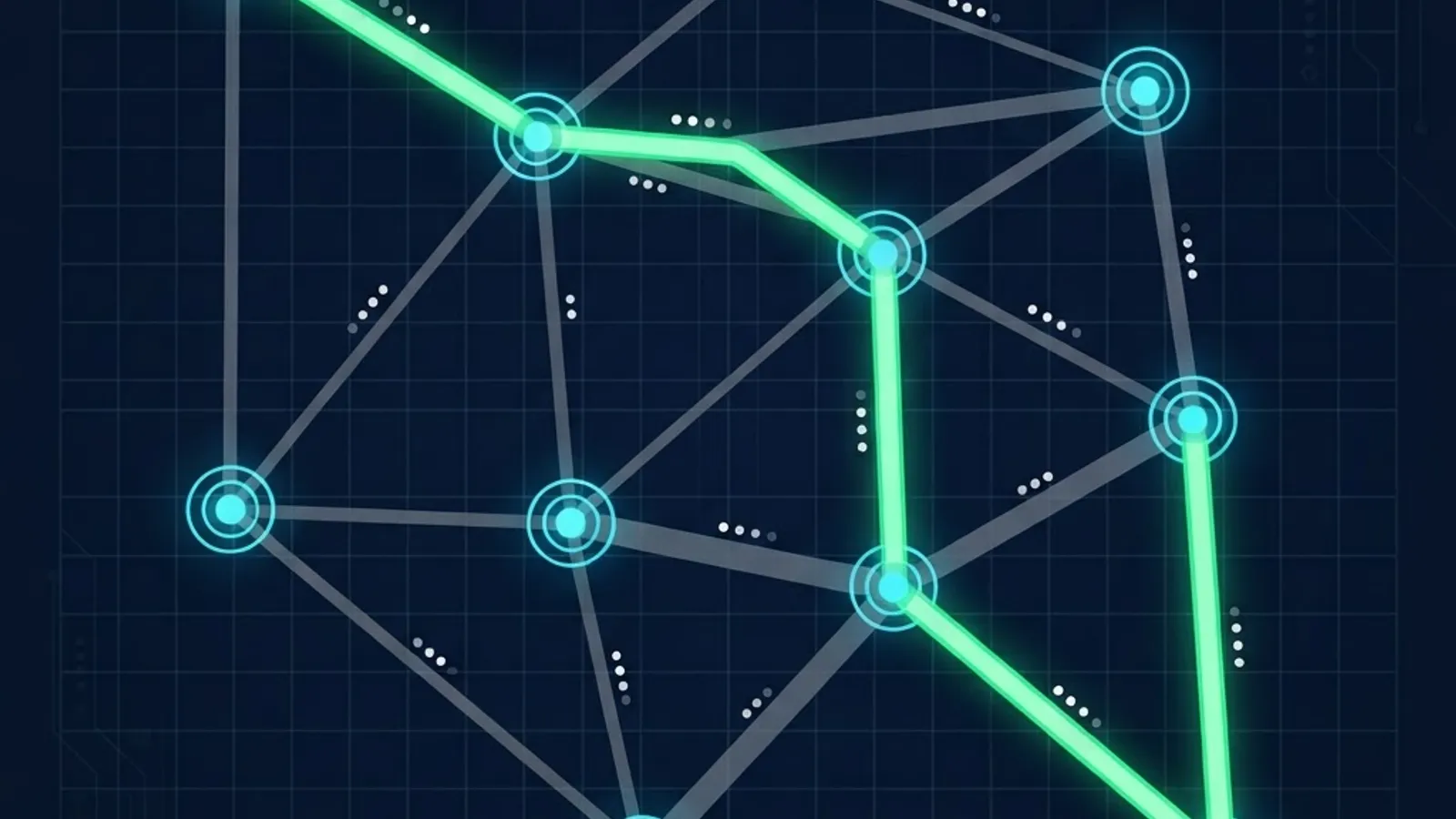
Use it when: actions have different real costs such as distance, time, money, or fuel.
6. Greedy Best-First Search
Greedy Best-First expands whichever node looks closest to the goal according to h(n) alone, ignoring the cost already paid. On open maps it is dramatically faster than UCS because it drives straight at the target instead of expanding concentric rings.
It is also neither optimal nor, in graph form without a closed set, complete. A single wall or detour can send it down a long path that looked promising. Treat greedy search as a speed-first heuristic for approximate answers, not a correctness tool.
7. A Star Search
A star evaluates f(n) = g(n) + h(n), balancing cost paid against cost estimated. With an admissible heuristic it is optimal, and with a consistent heuristic it never needs to reopen a closed node. It has been the default pathfinding algorithm in commercial games since the 1990s and remains the baseline in robotics motion planning.
Two practical rules decide whether your A star implementation is good. First, heuristic and movement rules must match: use Manhattan distance for 4-way grids and octile distance for 8-way grids, because Euclidean distance on a 4-way grid underestimates badly and expands far more nodes than necessary. Second, more informed admissible heuristics dominate weaker ones and expand strictly fewer nodes, which is why h = 0 collapses A star back into UCS.
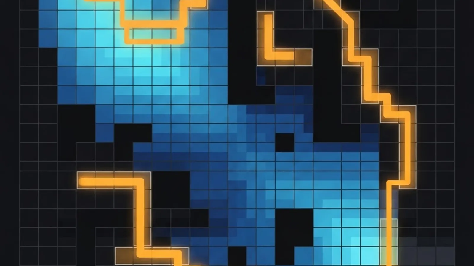
Use it when: you need the optimal weighted path and a decent heuristic exists.
8. Bidirectional Search
Bidirectional search runs two frontiers, one forward from the start and one backward from the goal, stopping when they meet. The complexity argument is the entire point: two searches of depth d/2 cost O(b^(d/2)) instead of O(b^d). At b = 10 and d = 6, that is roughly 2,000 nodes instead of 1,000,000.
It requires a well-defined single goal state and reversible actions, and the intersection test must be handled carefully to preserve optimality. When those conditions hold, no other structural trick delivers a comparable speedup for free.
9. Minimax With Alpha-Beta Pruning
Minimax handles adversarial search: you maximize, the opponent minimizes, and the value of a position propagates up the game tree. Raw minimax explores O(b^d) nodes, which is hopeless for real games.
Alpha-beta pruning discards branches that provably cannot influence the final decision. With ideal move ordering it reduces the effective cost to O(b^(d/2)), which doubles searchable depth in the same time budget. That is the difference between a club-level engine and a strong one. Modern engines layer on transposition tables, iterative deepening, and quiescence search, but alpha-beta remains the foundation.
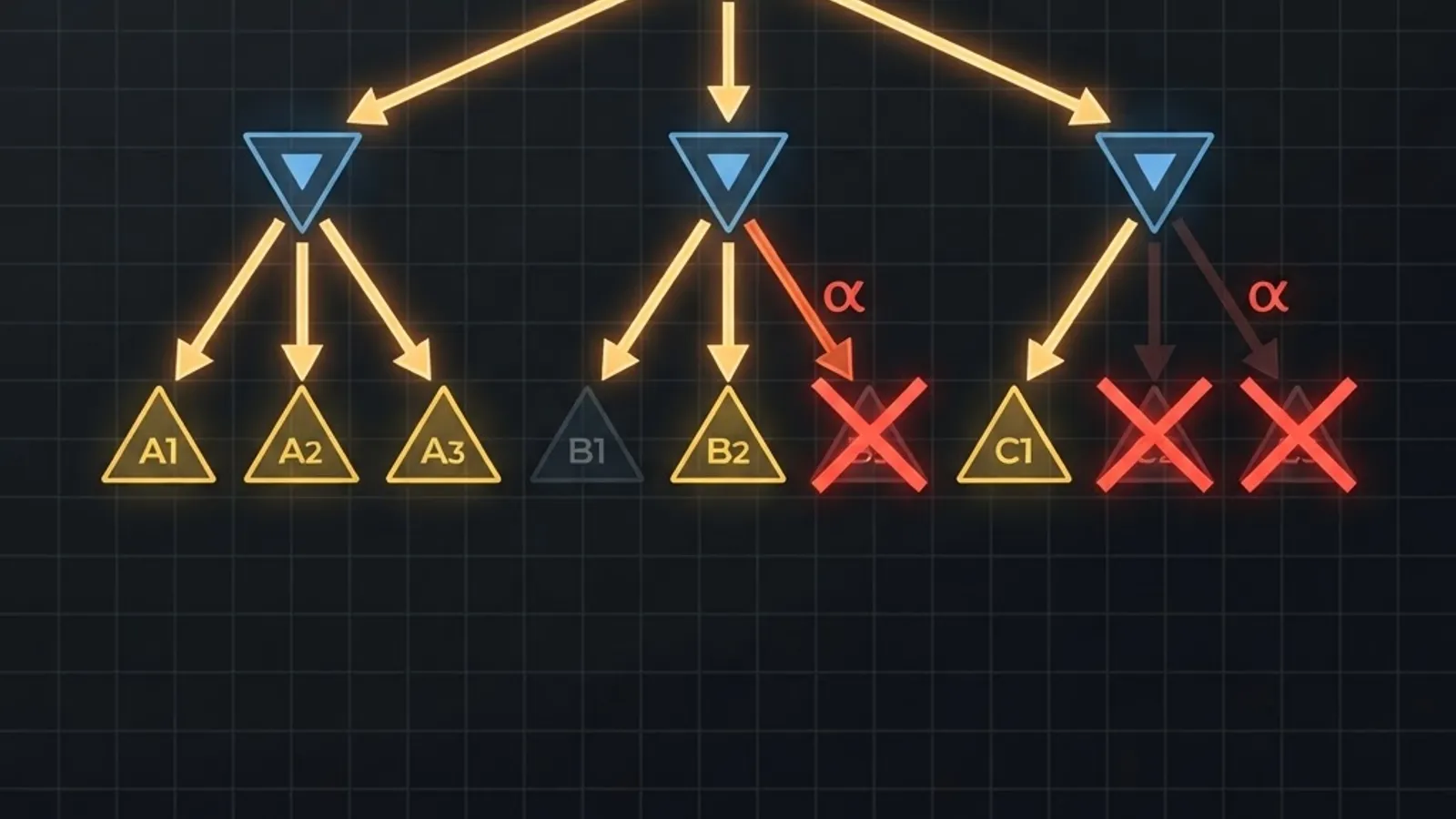
Use it when: two agents have directly opposed objectives and the state is fully observable.
10. Hill Climbing and Local Search
Hill climbing keeps a single current state and moves to the best neighbor until no neighbor improves. It uses constant memory and scales to state spaces far too large to enumerate, which is why local search dominates real optimization work such as scheduling, VLSI layout, and hyperparameter tuning.
Its failure modes are named and predictable: local maxima, plateaus, and ridges. The standard remedies are random restarts, sideways moves with a cap, stochastic neighbor selection, and simulated annealing, which accepts worsening moves with probability that decays over time. Learn hill climbing as the entry point to the entire metaheuristic family.
Comparison Table: Choose the Right Algorithm
| Algorithm | Complete | Optimal | Time | Space | Best Use Case |
|---|---|---|---|---|---|
| BFS | Yes | Yes, uniform cost | O(b^d) | O(b^d) | Shortest hop count |
| DFS | No | No | O(b^m) | O(bm) | Deep trees, low memory |
| DLS | No | No | O(b^L) | O(bL) | Fixed time budget |
| IDDFS | Yes | Yes, uniform cost | O(b^d) | O(bd) | Large trees, optimal needed |
| UCS | Yes | Yes | O(b^(1+C/e)) | High | Weighted edges |
| Greedy | No | No | O(b^m) | O(b^m) | Fast approximate routes |
| A star | Yes | Yes, admissible h | Exponential | High | Optimal pathfinding |
| Bidirectional | Yes | Yes, with BFS | O(b^(d/2)) | O(b^(d/2)) | Known single goal |
| Alpha-Beta | Yes | Yes, vs optimal play | O(b^(d/2)) best | O(bd) | Two-player games |
| Hill Climbing | No | No | Varies | O(1) | Huge optimization spaces |
How to Actually Learn These in the Right Order
The sequence matters more than the volume. Based on how these concepts build on each other, this order minimizes wasted effort:
- Implement BFS and DFS from scratch with an explicit queue and stack, never recursion, so the frontier data structure is visible.
- Add DLS, then IDDFS, and count nodes expanded to see the overhead argument yourself.
- Move to UCS with a priority queue and confirm goal-test-on-expansion behavior with a deliberately tricky weighted graph.
- Add h(n) to build Greedy, then A star, then break admissibility on purpose and watch optimality fail.
- Finish with alpha-beta on tic-tac-toe and hill climbing on 8-queens.
One habit separates students who retain this from those who do not: instrument every implementation to print nodes expanded, maximum frontier size, and path cost. Those three numbers turn abstract complexity classes into observable behavior, and they are exactly what an interviewer wants you to reason about.

Search fundamentals also transfer directly into production engineering. Recommendation ranking, retrieval pipelines, constraint-based scheduling, and agentic tool selection are all search problems wearing different clothes, which is why teams building AI workflow solutions still reason in terms of state spaces and cost functions. The ZoneTechify Team applies the same evaluation discipline, measuring expansions and cost rather than trusting intuition, when designing production AI systems.
Key Takeaways
- BFS is optimal only when all edge costs are equal, while UCS generalizes it to weighted graphs and is equivalent to Dijkstra's algorithm.
- IDDFS achieves BFS optimality with DFS memory, adding roughly 11 percent node overhead at branching factor 10.
- A star is optimal if and only if its heuristic is admissible, and never reopens closed nodes when the heuristic is consistent.
- Alpha-beta pruning with good move ordering cuts minimax from O(b^d) to about O(b^(d/2)), effectively doubling search depth.
- Bidirectional search reduces O(b^d) to O(b^(d/2)) but requires a known goal state and reversible actions.
- Hill climbing uses constant memory and is the gateway to simulated annealing and other metaheuristics.
Frequently Asked Questions (FAQ)
What is the difference between informed and uninformed search?
Uninformed search algorithms like BFS, DFS, and UCS use only the problem definition and path cost so far. Informed search algorithms like Greedy and A star additionally use a heuristic that estimates remaining distance to the goal, which lets them expand far fewer nodes on large state spaces.
Is A star always better than Dijkstra's algorithm?
Not always. A star reduces to Dijkstra when the heuristic returns zero, so it is never worse asymptotically. But A star needs a goal-specific heuristic. If you need shortest paths from one source to all nodes, or no useful heuristic exists, Dijkstra or UCS is the correct choice.
Which search algorithm should I learn first as a CS student?
Start with BFS and DFS implemented using an explicit queue and stack. Every other algorithm on this list is a modification of one of those two frontier strategies. Once you can trace their node expansion order by hand, UCS, IDDFS, and A star take far less time to absorb.
Why does DFS use less memory than BFS?
BFS stores an entire level of the tree in its frontier, which grows exponentially as O(b^d). DFS only stores the nodes along the current path plus their unexplored siblings, giving linear O(bm) space. That difference is why DFS handles deep search trees that would exhaust memory under BFS.
What makes a heuristic admissible in A star?
A heuristic is admissible when it never overestimates the true remaining cost to the goal. Straight-line distance is admissible for road networks because no real route is shorter than a straight line. Admissibility is the precise condition that guarantees A star returns an optimal path.
Are classical search algorithms still relevant with modern AI?
Yes. Beam search drives text generation in language models, Monte Carlo Tree Search powers game-playing systems, and A star variants run in robotics and logistics daily. Classical search provides the guarantees, cost accounting, and complexity vocabulary that learned models alone do not supply.